
广义加性模型算例
Published:
本算例展示三项内容:
- 先用默认的 LinearGAM 作为同方差基线;
- 再用 LinearGAM + FGLS 近似处理异方差;
- 对比两种预测区间在噪声随 $x$ 增大时的差异。
一、环境配置
conda create -n pyGAM python=3.11
conda activate pyGAM

pip install pygam==0.12.0
pip install seaborn==0.13.2
pip install jupyter==1.1.1
导入必要的库:
from matplotlib.ticker import MultipleLocator, AutoMinorLocator
import matplotlib.pyplot as plt
import seaborn as sns
import numpy as np

from pygam import LinearGAM
二、生成测试样本
本算例展示三项内容:
- 先用默认的 LinearGAM 作为同方差基线;
- 再用 LinearGAM + FGLS 近似处理异方差;
- 对比两种预测区间在噪声随 $x$ 增大时的差异。
生成测试样本:
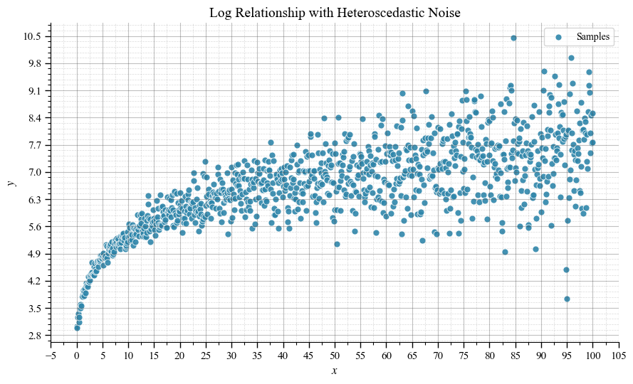
- 均值函数设为 $3 + \log(x + 1)$;
- 噪声标准差设为 $0.1(0.1x + 1)$,因此噪声会随 $x$ 增大而增大;
- 固定随机种子,保证 notebook 每次运行结果一致。
rng = np.random.default_rng(42)
x_samples = np.linspace(0, 100, 1000)
X = x_samples.reshape(-1, 1)

y_true = 3 + np.log(x_samples + 1)
noise_scale = 0.1 * (0.1 * x_samples + 1)
y_samples = y_true + rng.normal(0, noise_scale, size=x_samples.shape)
先定义统一的绘图辅助函数,并查看模拟样本。
def configure_plot_style():
    plt.rcParams["font.family"] = "Times New Roman"
    plt.rcParams["mathtext.fontset"] = "stix"


def apply_axis_style(ax, x_values, y_values, title, xlabel="$x$", ylabel="$y$"):
    x_step = max(1, int(np.max(x_values) / 20))
    y_range = max(float(np.max(y_values) - np.min(y_values)), 1.0)
    y_step = max(0.5, round(y_range / 10, 1))

    ax.xaxis.set_major_locator(MultipleLocator(x_step))
    ax.xaxis.set_minor_locator(AutoMinorLocator(2))
    ax.yaxis.set_major_locator(MultipleLocator(y_step))
    ax.yaxis.set_minor_locator(AutoMinorLocator(5))

    ax.grid(True, which="major", linestyle="-", linewidth=0.8, alpha=0.35, color="#4C4C4C")
    ax.grid(True, which="minor", linestyle="--", linewidth=0.5, alpha=0.2, color="#4C4C4C")
    ax.set_title(title, fontsize=14)
    ax.set_xlabel(xlabel, fontsize=12)
    ax.set_ylabel(ylabel, fontsize=12)
    ax.tick_params(axis="both", which="major", labelsize=11, length=6, width=1.0)
    ax.tick_params(axis="both", which="minor", length=3, width=0.8)


def plot_samples(ax, x_values, y_values, label="Samples", alpha=0.9):
    return sns.scatterplot(
        x=x_values, y=y_values,
        s=42, color="#2E86AB",
        edgecolor="white", linewidth=0.6, alpha=alpha,
        ax=ax, label=label
    )


configure_plot_style()
fig, ax = plt.subplots(figsize=(9, 5.5))
plot_samples(ax, x_samples, y_samples)
apply_axis_style(ax, x_samples, y_samples, "Log Relationship with Heteroscedastic Noise")
sns.despine()
plt.tight_layout()
三、同方差 vs 异方差GAM建模
3.1 同方差模型
接下来,采用GAM对数据进行拟合:
先给出同方差基线模型。这里的 LinearGAM 使用单一噪声尺度,因此适合作为对照,而不是最终的异方差解法。
gam_homo = LinearGAM(
    n_splines=10,
    spline_order=3,
    fit_intercept=True
).fit(X, y_samples)
绘制同方差基线模型的均值曲线、95% 置信区间(CI)和 95% 预测区间(PI)。
y_pred_homo = gam_homo.predict(X)
y_ci_homo = gam_homo.confidence_intervals(X, width=0.95)
y_pi_homo = gam_homo.prediction_intervals(X, width=0.95)

configure_plot_style()
fig, ax = plt.subplots(figsize=(9, 5.5))
plot_samples(ax, x_samples, y_samples)
ax.fill_between(x_samples, y_pi_homo[:, 0], y_pi_homo[:, 1], color="#8E9AAF", alpha=0.22, label="95% PI (homoscedastic)")
ax.plot(x_samples, y_pred_homo, color="#E76F51", linewidth=2.2, label="LinearGAM mean")
ax.fill_between(x_samples, y_ci_homo[:, 0], y_ci_homo[:, 1], color="#E76F51", alpha=0.25, label="95% CI (mean)")
apply_axis_style(
    ax,
    x_samples,
    np.concatenate([y_samples, y_pi_homo.ravel()]),
    "Homoscedastic LinearGAM: 95% CI vs 95% PI"
 )
ax.legend(frameon=False)
sns.despine()
plt.tight_layout()
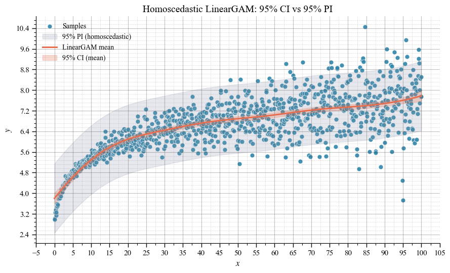
可以看到,基线模型的均值拟合是合理的,但其预测区间宽度变化较弱。原因是默认 LinearGAM 把噪声方差看作常数,因此不能显式表达“噪声随 $x$ 增大”的结构。
3.2 异方差模型
下面使用 LinearGAM + FGLS 做近似异方差建模。思路分三步:
- 先用基线模型得到残差;
- 对 $\log(\hat\varepsilon^2)$ 再拟合一个 GAM,估计方差函数;
- 用 $1/\hat\sigma^2(x)$ 作为权重重新拟合均值模型。
residuals_homo = y_samples - y_pred_homo

eps = 1e-10
log_res2 = np.log(residuals_homo ** 2 + eps)
var_gam = LinearGAM(
    n_splines=10,
    spline_order=3,
    fit_intercept=True
).fit(X, log_res2)

sigma_sq_fgls = np.exp(var_gam.predict(X))
weights_fgls = 1.0 / np.clip(sigma_sq_fgls, 1e-6, None)

gam_fgls = LinearGAM(
    n_splines=10,
    spline_order=3,
    fit_intercept=True
).fit(X, y_samples, weights=weights_fgls)

y_pred_fgls = gam_fgls.predict(X)
y_ci_fgls = gam_fgls.confidence_intervals(X, width=0.95)
sigma_fgls = np.sqrt(np.exp(var_gam.predict(X)))
z_score = 1.96
y_pi_fgls = np.column_stack([
    y_pred_fgls - z_score * sigma_fgls,
    y_pred_fgls + z_score * sigma_fgls,
])

print("FGLS 拟合完成:已同时得到均值模型和随 x 变化的噪声标准差估计。")
FGLS 拟合完成:已同时得到均值模型和随 x 变化的噪声标准差估计。
configure_plot_style()
fig, axes = plt.subplots(1, 2, figsize=(14, 5.5))

ax = axes[0]
plot_samples(ax, x_samples, y_samples, alpha=0.3)
ax.fill_between(x_samples, y_pi_homo[:, 0], y_pi_homo[:, 1], color="#A0A0A0", alpha=0.2, label="95% PI (homoscedastic)")
ax.fill_between(x_samples, y_pi_fgls[:, 0], y_pi_fgls[:, 1], color="#4E5A6E", alpha=0.4, label="95% PI (heteroscedastic)")
ax.plot(x_samples, y_pred_fgls, color="#E76F51", linewidth=2.3, label="FGLS mean")
ax.plot(x_samples, y_true, color="#1D3557", linewidth=1.8, linestyle="--", alpha=0.75, label="True mean")
apply_axis_style(
    ax,
    x_samples,
    np.concatenate([y_samples, y_pi_homo.ravel(), y_pi_fgls.ravel()]),
    "Prediction Interval: Homoscedastic vs Heteroscedastic"
 )
ax.legend(frameon=False)

ax = axes[1]
ax.plot(x_samples, noise_scale, color="#1D3557", linewidth=2.2, linestyle="--", label="True noise std")
ax.plot(x_samples, sigma_fgls, color="#E76F51", linewidth=2.2, label="Estimated noise std")
ax.fill_between(x_samples, 0, sigma_fgls, color="#E76F51", alpha=0.12)
apply_axis_style(
    ax,
    x_samples,
    np.concatenate([noise_scale, sigma_fgls]),
    "Noise Std: Truth vs FGLS Estimate",
    ylabel="Standard deviation"
 )
ax.legend(frameon=False)

sns.despine()
plt.tight_layout()
plt.show()
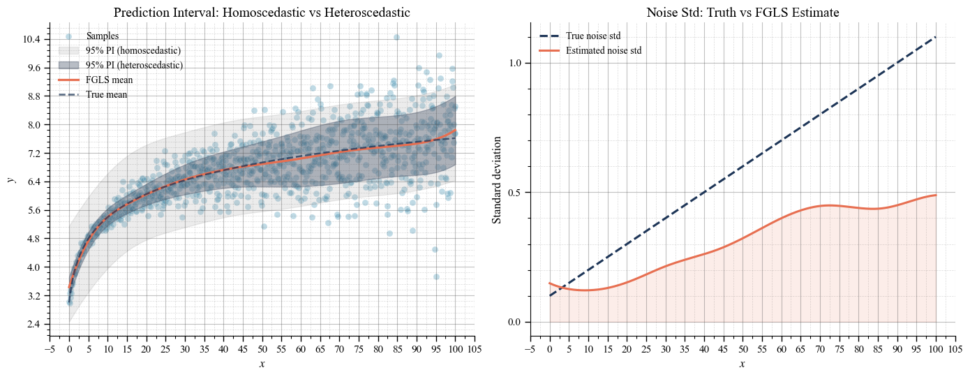
四、结论
- 默认
LinearGAM更适合作为同方差基线,它的 PI 宽度主要由单一噪声尺度决定; LinearGAM + FGLS通过“残差建模 + 加权重拟合”可以近似刻画异方差;- 在这个合成示例里,FGLS 给出的预测区间会随 $x$ 增大而变宽,同时估计出的噪声标准差也能较好追踪真实趋势。